Data Table
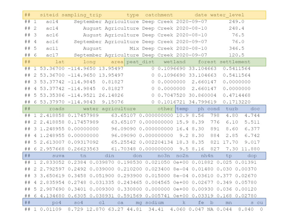
My data is comprised of 3 groups: (1) general catchment information shown in yellow, (2) land cover shown in green, and (3) water chemistry shown in blue. The siteid column indicates the sampling unit: 55 catchments that are sampled six times over the 2020-2021 time period. Because I am interested in how human land use affects water quality, the response variables are DOC, N species (TN, DIN, DON, NO3-N, NO2-N, and NH4-N), and P species (TP, DOP, and PO4-P). The predictor variables include land cover variables (continuous percentages based on GIS analysis) and ancillary water chemistry parameters such as temperature, pH, conductivity, turbidity, and other ions.
Table 1 Snapshot of my data frame in R. Columns highlighted in yellow indicate general catchment info. Green columns indicate land cover variables. Blue columns indicate water chemistry variables.
Graphical Data Exploration
|
Carbon, nitrogen, and phosphorous are the water quality parameters that I am monitoring in this study. For carbon, I am monitoring DOC, which is a bulk measurement of all organic forms of carbon that pass through a certain filter size (0.7 μm in the present study). Nitrogen and phosphorous, however, were measured as total forms and then were also divided into their primary ions and molecules. In Fig. 6, I show how the total fractions of nitrogen and phosphorous are divided on average into their various species for each catchment. For nitrogen, this shows that ammonium is especially high in disturbed sites, but the majority of nitrogen in the catchments is in the form of dissolved organic nitrogen. For phosphorous, the dominant form is phosphate, and there is little relationship between disturbance and phosphorous concentration.
As you will notice, there are a few catchments that consistently have high concentrations of nutrients and do not neatly fit my hypothesis that peatland disturbance is the main driver of nutrient conditions. I carefully examined these data to make sure that they were not simple sampling or data entry errors, and to the best of my knowledge these data are correct. Including the water quality parameters mentioned above, my main variables of interest are disturbed and pristine peatlands, and agriculture. Fig. 7 shows the distribution, correlation coefficients, and biplots among these variables. For the sake of space, I did not include figures for the entire water quality dataset. In this study, disturbed peatlands are the exception rather than the rule, and the distribution of % Disturbed Peat is heavily right-skewed with many subcatchments without any harvested peatland influence. % Wetland (a measure of the pristine peatlands in the area) has a bi-modal, right-skewed distribution showing the prevalence of wetlands in this landscape. % Agriculture has a more bell-shaped, normal distribution which also shows that heavy agricultural influence in the area. There is a negative correlation (Pearson correlation = -0.62) between % Wetland and % Agriculture, indicating that when wetlands dominate the landscape agriculture is not present, and vice versa. DOC has a slightly right-skewed, normal distribution with a mean value of 48.31 mg/L. This is well above the recommended DOC concentration guideline (7.90 mg/L) for the preservation of aquatic life in the North Saskatchewan River where Tomahawk and Deep Creek drain [20]. Ammonium (NH4) concentrations are heavily right-skewed with a mean value of 0.23 mg/L. The recommended ammonium guideline is ~0.018 mg/L, though this value depends on pH and temperature. Ammonium is also strongly correlated with % Disturbed Peat (Pearson correlation = 0.78). DIN is the sum of inorganic N species nitrate, nitrite, and ammonium. DIN and ammonium are strongly correlated (Pearson correlation = 0.88) indicating that the majority of DIN is ammonium. Phosphate, the inorganic and most bioavailable form of P, has a right-skewed distribution with a mean concentration of 0.17 mg/L. It is highly correlated with total phosphorus (TP; Pearson correlation = 0.92) which has a recommended guideline not to exceed 0.10 mg/L. Though P is not toxic to humans, an overabundance in aquatic systems can trigger algal blooms [21], so maintaining TP concentrations below this guideline is advised.
|

Fig. 6 The composition of total N and total P by average concentration of N and P species for each catchment. Catchments are ordered by the amount of peatland disturbance within their catchment (most disturbed to least disturbed).

Fig. 7 Exploratory data analysis of a subset of the geospatial and water chemistry data. Histograms down the middle show disturbutions of the data, the bottom left corner shows scatter plots between variables and the top right corner shows Pearson correlations. The larger the correlation the larger the text. Asterisks show significant correlations (* = 0.05, ** = 0.01, *** = <0.001).
|
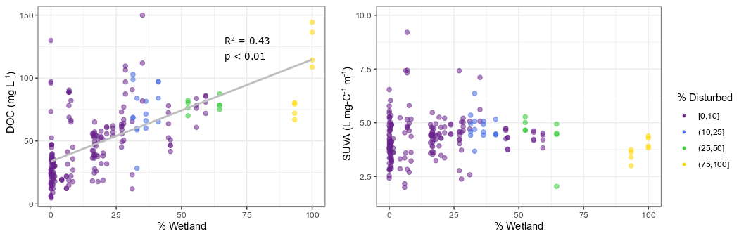
Fig. 8 The relationship between cumulative wetland cover (pristine and disturbed) and dissolved organic carbon (DOC) concentration and quality (SUVA). Points are colored by the proportion of peatland disturbance in the catchments. DOC concentration has a positive relationship with wetland cover that shows that peatland disturbance may not have a large effect on DOC concentrations. SUVA (a proxy of DOC quality) shows no relationship with wetland cover, and disturbance exhibits similar patterns to other pristine wetlands.
However, on closer inspection, the relationship between peatland disturbance and DOC may not be quite as certain. Fig. 8 shows the relationship between DOC and specific ultraviolet absorbance of the DOC (SUVA; a proxy for DOC quality) with overall wetland cover. Each point is colored by the amount of disturbance in the catchments, and in the concentrations of DOC in the disturbed sites is consistent with the linear relationship of wetland generally. In other words, the elevated concentrations of DOC in disturbed peatland land cover classes could be an artifact of sampling bias. When selecting sites, we tried to get a diverse number of watersheds with small headwater catchments predominantly covered by disturbed peatland, pristine peatlands, and agriculture. However, because of private land access we were not able to sample 100% pristine peatland subcatchments to compare to the 100% disturbed peatland subcatchments. Perhaps if we had measured a catchment with 100% pristine peatland land cover then maybe we could draw a more definitive conclusion. However, that is not the case, so the DOC data must be carefully interpreted. The SUVA plot further supports this finding, because there is no difference between SUVA measured in disturbed and pristine sites. Therefore, our data suggest that disturbance may increase DOC concentrations in receiving waterbodies, but more research is needed to reach a definitive conclusion.
|
However, ammonium shows that disturbance does make a difference. In Fig. 9, the same relationship is explored as in the figures above. Ammonium is consistently low, with little variability, in the pristine sites until the highly disturbed sites, where concentrations are elevated beyond what could be expected. Not only does this finding point to excess nitrogen delivery to downstream waterbodies, but it also points to oxidation of peat organic matter playing a role in observed nutrient conditions and supports the idea that DOC may also be elevated in disturbed sites.
|
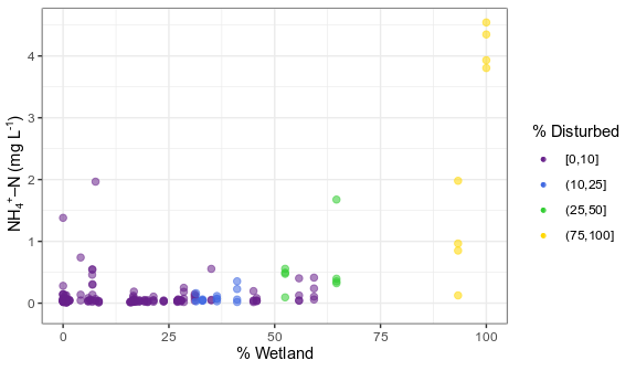
Fig. 9 The relationship between cumulative wetland cover (pristine and disturbed) and ammonium (NH4-N) concentrations. Points are colored based on the proportion of peatland disturbance in the catchment.
|
|
To use predictive models to disentangle the influence of geospatial catchment data on stream water chemistry, I used Random Forest regression models to predict DOC, DIN, and TP concentrations. However, Random Forest models are sensitive to correlated explanatory variables and will split their importance. Therefore, prior to running the models I generated correlation plots of the geospatial catchment data to check for highly correlated variables (Fig. 10). % Agriculture and % Wetland were the most highly correlated variables (Spearman correlation = -0.66), but because agriculture and wetlands are both important predictors of stream water quality and because the correlation coefficient was sufficiently low, I did not remove either of these variables from the models. The next most correlated variables were % Agriculture and % Roads. This is expected because this study is located in rural Alberta where roads are constructed primarily for accessing agricultural land. I removed % Roads from the models and model performance was not affected (< 1% change in RMSE and OOB R-squared values). Similarly, % Settlement, % Water, and % Other were correlated with catchment area and account for a small fraction of the landscape (mean = 7.43%, min = 0.90%, max = 30.07%). Therefore, I removed % Settlement, % Water, and % Other from the model and model performance was not affected (< 1% change in RMSE and OOB R-squared values).
|

Fig. 10 Spearman correlation plot of geospatial catchment characteristics. Cool colors show positive correlations and warm colors show negative correlations. The strongest correlations (both positive and negative) are labelled with correlation coefficients for context.
|
