Data CollectionWater chemistry
Water samples were collected from 55 subcatchments using a synoptic sampling design such that all 55 sites were sampled in 2–3 consecutive days with consistent weather conditions to minimize changes in water chemistry and flow. We were able to complete 5 synoptic samplings in 2020 and 2021 to capture seasonal and temporal variability in nutrient dynamics, including the spring freshet, summer baseflow, and storm events [14, 15]. Surveys were conducted monthly from June-September 2020, and during the spring snowmelt in March 2021. Water samples were collected from the midpoint of small streams and from the banks of larger streams. Turbidity, pH, electrical conductivity, and water temperature were analyzed in the field. Turbidity was analyzed using a portable 2020i Turbidity Meter (LaMotte, USA). pH, EC, and water temperature were measured using a handheld multiparameter probe (Hanna, USA). Readings were recorded after they had stabilized, usually after approximately one minute of submerging the probe in the sample. Both analyzers were calibrated in the morning before each sampling outing. Stream water samples were immediately filtered in the field using 0.7 μm Whatman GF/F filters. Samples for DOC and nutrient analysis were filtered into pre-rinsed, acid-washed 60 mL glass amber bottles. Samples were stored on ice until returning to the lab. DOC samples were acidified within 24-hours of collection and all samples were stored refrigerated at 4⁰C until analysis. DOC samples were analyzed on a Shimadzu TOC-L CPH Model Total Organic Carbon Analyzer with an ASI-L and TNM-L (Shimadzu, China). Dissolved sulfate, nitrate, nitrite, chloride, phosphate, and ammonium, were analyzed with a Thermo Gallery Plus Beermaster Autoanalyzer (Thermo Fisher Scientific, Finland). Dissolved metals (Na, K, Ca, Mg, Fe, B, Mn, Zn, Cu, Mo, and Ni), total sulfur, and total phosphorus were analyzed with a Thermo iCAP6300 Duo inductively coupled plasma-optical emission spectrometer (ICP-OES, Thermo Fisher Corp., United Kingdom). Samples were analyzed within one week. Geospatial catchment data All catchments were delineated in ArcGIS using the Alberta Provincial 25 m Raster and Base Watersheds digital elevation model and were manually adjusted based on road and culvert diversions. Catchment characteristics were extracted from the Alberta Biodiversity Monitoring Institute (ABMI) Human Footprint Inventory and Alberta Merged Wetland Inventory geospatial datasets [16, 17]. Land use classifications were manually characterized by continuous geospatial catchment data and Google Earth imagery. These classifications were used to divide the subcatchments into their dominant land use and land cover classes. Small catchments (< 30 square kilometers) were relatively simple to characterize because of their size. Larger subcatchments along the mainstem of the streams were more difficult to classify and were lumped into the “Mixed” catchment category. |

Fig. 4 Photo example of water chemistry sampling in the field.
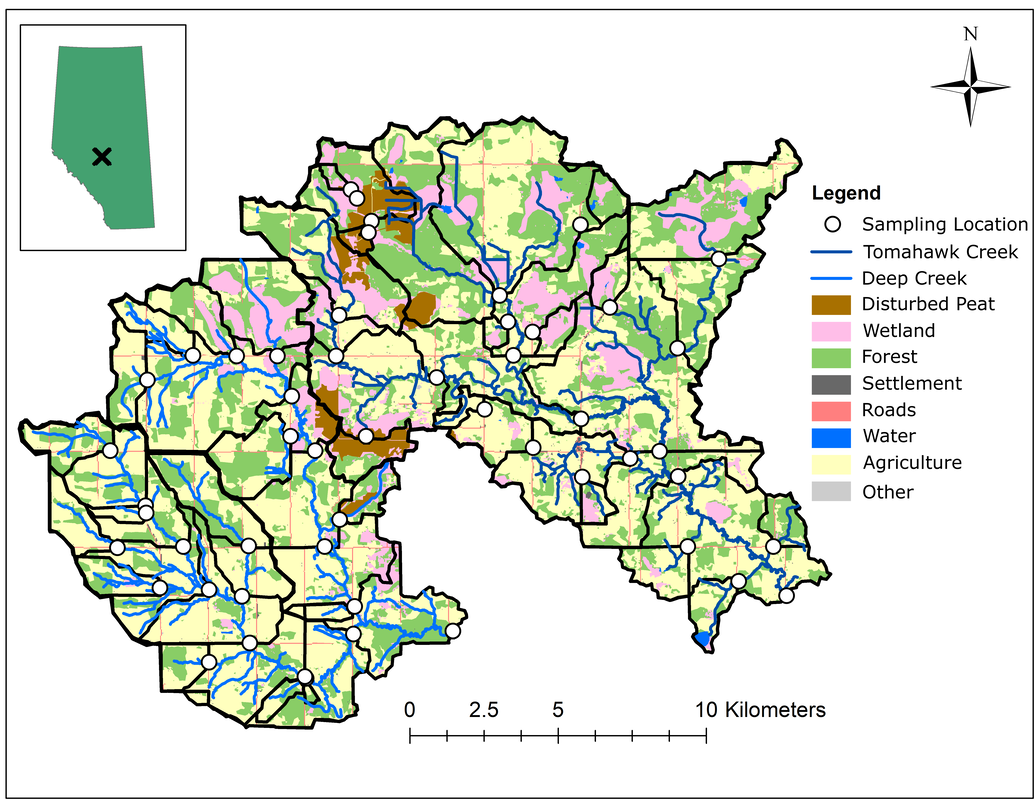
Fig. 5 Map of synoptic sampling locations near Seba Beach, Alberta, Canada delineated by black hexagons. The Deep Creek Catchment lies to the west and is dominated by cropland, forests, with some wetlands including disturbed peatlands to the east. The Tomahawk Creek Catchment lies to the east and is dominated by wetlands and disturbed peatlands in the north, and forests and cropland to the south near the catchment outlet.
|
Statistical Analysis
I used a multivariate statistical approach called nonmetric multidimensional scaling (NMDS) to reduce complexity in the catchment and water quality data. NMDS is a distanced-based ordination technique that reduces complexity in the dataset by describing multiple variables as components. NMDS is a robust technique that handles normal and non-normally distributed data. For this ordination, I first ordinated the geospatial catchment data and added ellipses to show land classification groupings. I then ran an ordination for the water chemistry data (DOC, N, and P) and added those vectors on top of the geospatial catchment ordination.
Random Forest regression models were used to predict stream water concentrations of DOC, N, and P using geospatial catchment data. Random Forest models use bootstrapped regression trees that randomly leave out explanatory variables and create forests to predict the response variable [18]. This method is statistically robust and does not require normally-distributed data. However, models can be sensitive to over-parametrization and may be adversely impacted by highly correlated explanatory variables. Therefore, Spearman correlations among explanatory variables were analyzed prior to analysis and correlated variables were removed from the analysis (see Fig. 10 in the Data tab). Models were trained on 80% of the data and predictions were generated and validated against the remaining test data (20% of the original data). Root Mean Square Error (RMSE) and out-of-bag (OOB) R-squared values are reported for each model.
Two-way analysis of variance (ANOVA) and Tukey Honest Significant Differences (HSD) tests were used to test for significant differences among land use and land cover classes. This analysis was run on log-transformed data, and tests for significance were based on p-values < 0.05.
All statistical and graphical analysis was conducted in R version 3.6.1 [19].
